Pyramid metanetwork example using ‘metanetwork’
Marc Ohlmann
2023-05-22
Source:vignettes/pyramid.Rmd
pyramid.RmdPreliminaries
This vignette illustrates ‘metanetwork’ through a pyramid network example. The packages required to run the vignette are the following:
Generating pyramid data set
Generating the metaweb an representing it using ‘ggnet2’
We first generate a pyramid network using ‘igraph’ and represent it using ‘ggnet2’
library(igraph)
library(network)
library(intergraph)
library(GGally)

n = 5
#generate a lattice
g = igraph::make_lattice(dim = 2,length = n,directed = T)
#deleting nodes and edges
nodes_to_rm = c()
for (k in 1:(n-1)){
  nodes_to_rm = c(nodes_to_rm,((k-1)*n+1):(k*n - k))
}
g = delete_vertices(g,nodes_to_rm)
g = delete_edges(g,c("7|12","8|13","9|14","2|5"))
V(g)$name = LETTERS[1:vcount(g)]
#representing the lattice using ggnet package
network = asNetwork(g)
ggnet2(network, arrow.size = 7,size = 3 ,arrow.gap = 0.025, label = T)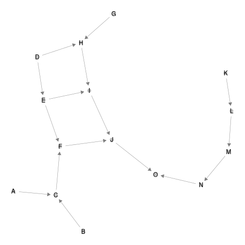
plot of chunk pyramid_build
Notice that ‘ggnet2’ default layout algorithm (Fruchterman-Reingold algorithm, a force directed algorithm) is non-reproducible. Moreover, x-axis and y-axis do not have any ecological interpretation.
ggnet2(network, arrow.size = 7,size = 3 ,arrow.gap = 0.025, label = T)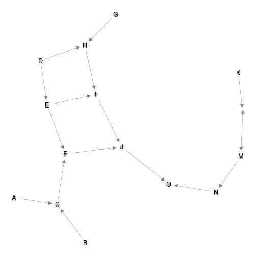
plot of chunk unnamed-chunk-1
Building a metanetwork object
From the lattice metaweb and abundance table, build a S3 object of
class ‘metanetwork’ using build_metanetwork
#building metanetwork object
meta0 = build_metanet(metaweb = g,abTable = presence)
class(g)
## [1] "igraph"
class(meta0)## [1] "metanetwork"method print prints a summary of the considered
metanetwork.
print(meta0)## metaweb has 15 nodes and 16 edges
## 3 local networks
## single resolution availableHandling metanetworks
the class ‘metanetwork’
A ‘metanetwork’ object consists in a list of ‘igraph’ objects:
- metaweb, the metaweb used to build the metanetwork, an ‘igraph’
object with node attribute
$abindicating the local relative abundance of each node and graph attribute$nameindicating"metaweb" - local networks, a list of ‘igraph’ objects with node attribute
$abindicating the local relative abundance of each node in each network and graph attribute$nameindicating local network names, that is rownames of the abundance table.
meta0$b$name## [1] "b"
meta0$metaweb$name## [1] "metaweb"##
## 0.0833333333333333
## 12##
## 0.032258064516129 0.0645161290322581 0.0967741935483871
## 3 8 4Metaweb node relative abundances are the mean of the local relative
abundances. Additional objects like abTable or
trophicTable can be included in a ‘metanetwork’ object
Computing trophic levels
‘metanetwork’ package enables 2D network representation with x-axis
equals to trophic levels. To compute trophic levels, ‘metanetwork’
implements the method, based on Laplacian matrix, described in MacKay et
al. 2020.
The metaweb needs to be connected for trophic levels to be unique. Local
networks can however be disconnected (see Ref). A method
compute_TL allows computing trophic levels and storing it
as node attribute $TL of each network.
#compute trophic levels for metaweb and local networks
meta0 = compute_TL(meta0)
V(meta0$metaweb)$name
## [1] "A" "B" "C" "D" "E" "F" "G" "H" "I" "J" "K" "L" "M" "N" "O"
V(meta0$metaweb)$TL## [1] 0.000000e+00 0.000000e+00 1.000000e+00 4.440892e-16 1.000000e+00 2.000000e+00 4.440892e-16 1.000000e+00 2.000000e+00 3.000000e+00
## [11] 0.000000e+00 1.000000e+00 2.000000e+00 3.000000e+00 4.000000e+00Representing metanetworks
‘metanetwork’ implements a layout algorithm, ‘TL-tsne’, specifically designed for trophic networks, based on trophic levels and on dimension reduction of graph diffusion kernel.
Diffusion graph kernel
Diffusion kernel is a similarity matrix between nodes according to a diffusion process. Let \(G\) be a directed network, \(\mathbf{A}\) its adjacency matrix and \(\mathbf{D}\) its degree diagonal matrix. The laplacian matrix of \(G\) is defined as:
\[\begin{equation} \mathbf{L} = \mathbf{D} - \mathbf{A} - \mathbf{A}^{T} \end{equation}\]
The diffusion kernel is then defined as (Kondor & Lafferty, 2002):
\[\begin{equation} \textbf{K} = \exp(-\beta\mathbf{L}) = \sum_{k \geq 0} \frac{(- \beta\mathbf{L})^k}{k!} \end{equation}\]
with \(\beta\) a positive parameter. Diffusion kernel measures similarity between pairs of nodes by taking into account paths of arbitrary length. It does not restrict to direct neighbors.
beta parameter
\(\beta\) is the single parameter of the diffusion kernel. It controls the weight given to the different paths in the diffusion kernel. It is also analogous to the diffusion constant in physics. We’ll see through examples its importance in squeezing networks.
ggmetanet function
The main metanetwork representation function is
ggmetanet. It allows representing metaweb and local
networks using ggnet and both layout algorithms.
ggmetanet plots the metaweb of the current metanetwork by
default.
#ggmetanet#
ggmetanet(metanetwork = meta0,beta = 0.1)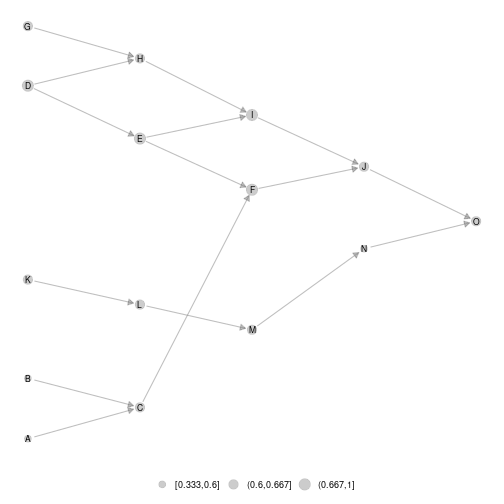
plot of chunk unnamed-chunk-7
#ggmetanet#
ggmetanet(metanetwork = meta0,beta = 0.45)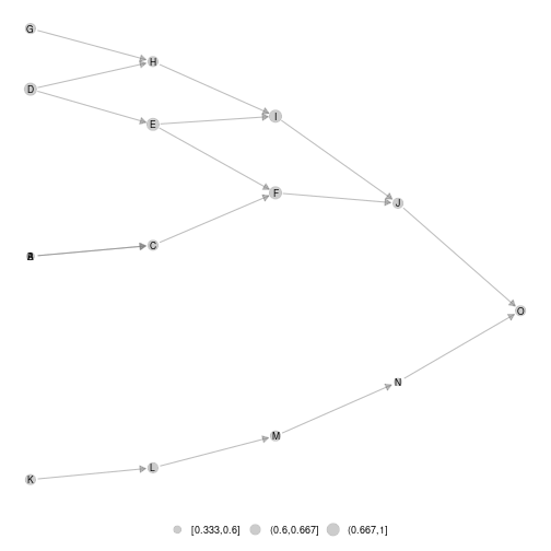
plot of chunk unnamed-chunk-8
ggmetanet can also represent local networks (with
specific layout)
ggmetanet(g = meta0$b,beta = 0.1,metanetwork = meta0)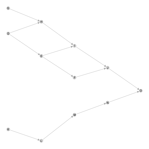
plot of chunk unnamed-chunk-9
Increasing beta squeeze y-axis
ggmetanet(g = meta0$b,beta = 1,metanetwork = meta0)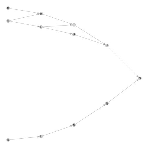
plot of chunk unnamed-chunk-10
Moreover, it clusters nodes belonging to different ‘branches’. They become more and more similar when beta is increased.
Representing disconnected networks
If the metaweb needs to be connected, local networks can be disconnected due to sampling effects. In that case, trophic levels are computed using metaweb trophic levels. The basal species of each connected component has a trophic level equals to its value in the metaweb.
ggmetanet(g = meta0$a,beta = 0.45,metanetwork = meta0)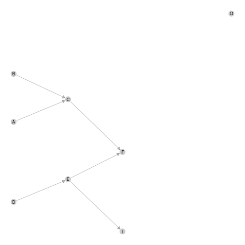
plot of chunk unnamed-chunk-11
diff_plot function
In order to compare local networks, a diff_plot function
is implemented. It colors nodes according to their presence/absence or
variation in abundance in both networks.
diff_plot(g1 = meta0$a,g2 = meta0$b,beta = 0.1,mode = 'TL-tsne',metanetwork = meta0)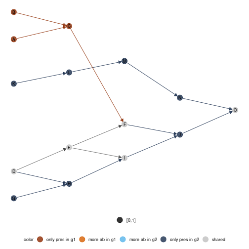
plot of chunk unnamed-chunk-12
Changing ggnet configuration parameters
In order to fine tune network plots, it is possible to modify
ggnet parameters in metanetwork. An object
ggnet.default is stored and wraps the different
visualisation parameters. Change it to modify the plot.
ggnet.custom = ggnet.default
ggnet.custom$edge.size = 3*ggnet.default$edge.size
ggnet.custom$label.size = 7
ggmetanet(beta = 0.1,metanetwork = meta0,
          ggnet.config = ggnet.custom)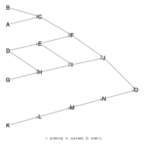
plot of chunk unnamed-chunk-13
Attaching layout
For network representation reproducibility and to gain computation
time, we recommend to store ‘TL-tsne’ layout after computation. To do
so, use the method attach_layout. Once the layout computed,
it is attached to the network as node attribute.
#for the metaweb
meta0 = attach_layout(meta0,beta = 0.1)
V(meta0$metaweb)$layout_beta0.1
## [1] -10.5245709 0.5715783 -4.6297208 30.2718230 18.7743114 7.3023306 43.1058371 36.1900901 23.8856698 12.6402267 -44.7744167
## [12] -38.1999701 -31.4062122 -24.7935220 -18.4134542
#for a local network
meta0 = attach_layout(metanetwork = meta0,g = meta0$a,beta = 0.1)
V(meta0$metaweb)$layout_beta0.1
## [1] -10.5245709 0.5715783 -4.6297208 30.2718230 18.7743114 7.3023306 43.1058371 36.1900901 23.8856698 12.6402267 -44.7744167
## [12] -38.1999701 -31.4062122 -24.7935220 -18.4134542Then, any call of ggmetanet or
vismetaNetwork will use the computed layout for the desired
\(\beta\) value.
ggmetanet(meta0,beta = 0.1)
plot of chunk unnamed-chunk-15
Using that way, network representation is reproducible.
#calling again ggmetanet
ggmetanet(meta0,beta = 0.1)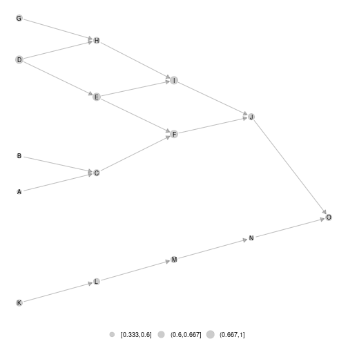 Once the layout computed for the
metaweb, it can be used to represent local network or difference network
using
Once the layout computed for the
metaweb, it can be used to represent local network or difference network
using layout_metaweb = T
#ggmetanet
ggmetanet(meta0,beta = 0.1,layout_metaweb = T)
plot of chunk unnamed-chunk-17
ggmetanet(g = meta0$a,metanetwork = meta0,beta = 0.1,layout_metaweb = T)
plot of chunk unnamed-chunk-17
ggmetanet(g = meta0$b,metanetwork = meta0,beta = 0.1,layout_metaweb = T)
plot of chunk unnamed-chunk-17
ggmetanet(g = meta0$c,metanetwork = meta0,beta = 0.1,layout_metaweb = T)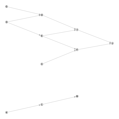
plot of chunk unnamed-chunk-17
#diffplot
diff_plot(meta0,meta0$a,meta0$b,beta = 0.1,layout_metaweb = T)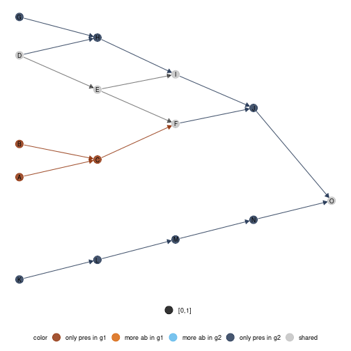
plot of chunk unnamed-chunk-17
Computing network indices and metrics
Besides network representation, ‘metanetwork’ package can compute usual network metrics (weighted connectance, mean and max trophic level, mean shortest path length). Network diveristy and dissimilarity indices based on Hill numbers are also implemented in order to quantitatively compare local networks.
  #computing network metrics
  compute_metrics(meta0)
## connectance mean_TL max_TL mean_shortest_path_length
## metaweb 0.08428720 1.333333 4 2.069767
## a 0.09375000 1.250000 4 1.400000
## b 0.09027778 1.583333 4 1.968750
## c 0.09090909 1.181818 3 1.550000The metaweb is less connected than local networks but have the
highest mean shortest path length. We now compute network diversity
indices based on Hill numbers (cf. Ohlmann et al. 2019). The indices are
based on node and link abundances are can be partitionned in \(\alpha\)-diversity, \(\beta\)-diversity and \(\gamma\)-diversity. A viewpoint parameter
\(q\) allows giving more weight (see
compute_div documentation)
#computing diversities
compute_div(meta0)
## $nodes
## $nodes$Gamma
## [1] 14.1607
##
## $nodes$mean_Alpha
## [1] 10.18329
##
## $nodes$Beta
## [1] 1.390582
##
## $nodes$Alphas
## a b c
## 8 12 11
##
##
## $links
## $links$Gamma
## [1] 14.53731
##
## $links$mean_Alpha
## [1] 9.502308
##
## $links$Beta
## [1] 1.529872
##
## $links$Alphas
## a b c
## 6 13 11Moreover, pairwise dissimilarity indices (both on nodes and links)
are also implemented in metanetwork (see compute_dis
documentation).
#computing pairwise dissimilarities
compute_dis(meta0)
## $nodes
## a b c
## a 0.0000000 0.4942966 0.4699751
## b 0.4942966 0.0000000 0.1299762
## c 0.4699751 0.1299762 0.0000000
##
## $links
## a b c
## a 0.0000000 0.6712475 0.5174744
## b 0.6712475 0.0000000 0.1650477
## c 0.5174744 0.1650477 0.0000000In this case, we see that links dissimilarities are higher than node dissimilarities. Indeed, absent nodes from the metaweb might lead to the absence of several edges.
References
Kondor, R. I., & Lafferty, J. (2002, July). Diffusion kernels on graphs and other discrete structures. In Proceedings of the 19th international conference on machine learning (Vol. 2002, pp. 315-322).
MacKay, R. S., S. Johnson, and B. Sansom. “How directed is a directed network?.” Royal Society open science 7.9 (2020): 201138
Ohlmann, M., Miele, V., Dray, S., Chalmandrier, L., O’connor, L., & Thuiller, W. (2019). Diversity indices for ecological networks: a unifying framework using Hill numbers. Ecology letters, 22(4), 737-747.