Norway soil metanetwork data set
Norway soil metanetwork dataset was extracted from Calderon-Sanou et al. 2021. It consists in a soil expert knowledge metaweb that contains \(40\) tropho-functional groups and \(204\) interactions. Tropho-functional groups have abundance data built from eDNA data in disturbed and non-disturbed sites by moth outbreaks. This dataset also contains a trophic table that contains broader taxonomic and functional informations on groups.
In this vignette, we aim at represent metaweb at different aggregation levels and compare local networks with layouts provided by ‘metanetwork’.
Loading the dataset
## [1] "metanetwork"
print(meta_norway)## metaweb has 40 nodes and 204 edges
## 2 local networks
## available resolutions (not computed) are: trophic_group trophic_class taxa
plot_trophic_table function
Trophic table describes nodes memberships in higher relevant groups.
In angola dataset, two different taxonomic resolutions are available.
Networks can be handled and represented at trophic class or trophic
group level.
The plot_trophic_table function allows representing the
tree describing species memberships.
ggnet.custom = ggnet.default
ggnet.custom$label.size = 2
plot_trophicTable(meta_norway,res = c('trophic_group','trophic_class'),ggnet.config = ggnet.custom)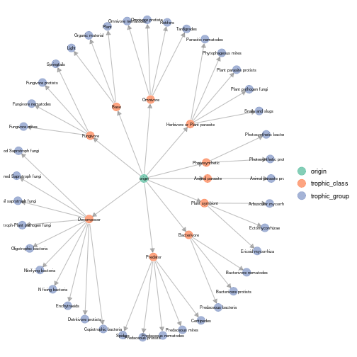
plot of chunk norway_plot_trophic_table
append_agg_nets method
The method append_agg_nets allows computing and
appending aggregated networks (at the different available resolutions
shown by plot_trophic_table) to the current
metanetwork.
meta_norway = append_agg_nets(meta_norway)
print(meta_norway)
## metaweb has 40 nodes and 204 edges
## 2 local networks
## available resolutions are: trophic_group trophic_class taxaRepresent the metaweb at several resolutions
Representing aggregated networks, adding a legend to networks
Once computed, ggmetanet function allows representing
aggregated networks and legending local networks using trophic table
using ‘ggnet’ visualisation. Do not forget to first compute trophic
levels. Computation of ‘TL-tsne’ layout is done ggmetanet
function.
meta_norway = compute_TL(meta_norway)
ggmetanet(g = meta_norway$metaweb_trophic_class,beta = 0.2,metanetwork = meta_norway)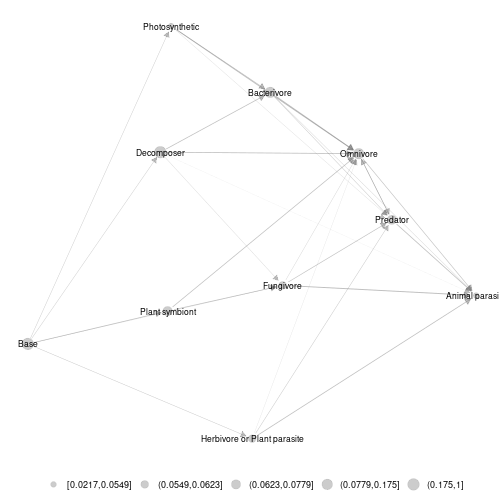
plot of chunk norway_metaweb_trophic_class
Node sizes are proportional to relative abundances. Trophic table allows adding a legend to network at the finest resolution.
ggnet.custom = ggnet.default
ggnet.custom$label.size = 2
ggmetanet(g = meta_norway$metaweb,beta = 0.006,legend = 'taxa',metanetwork = meta_norway, ggnet.config = ggnet.custom)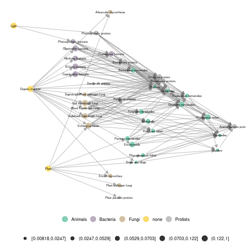
plot of chunk norway_metaweb
The metaweb has two basal resources: plant and organic material. They have the lowest x-axis values in the ‘TL-tsne’ layout. The channel starting from plants corresponds to the green energy channel while the channel starting from organic materials is the brown channel. Importantly, we observe from our network representation that bacterial and fungal paths are separated in the brown channel. It means that they are linked to separated paths higher up in the network (e.g. bacterivore and fungivore groups)
Attaching layout
Since TL-tsne layout is stochastic and requires (a bit
of) computation times, saving and using the the same layout (for a given
\(\beta\) value) is recommended.
Moreover, it makes easier visual network analysis and comparison since
it is fixed. attach_layout function allows saving computed
layouts by attaching them as a node attribute.
#attaching 'TL-tsne' layout to the metaweb
meta_norway = attach_layout(metanetwork = meta_norway,beta = 0.006)
#TL-tsne layout is stored as node attribute
igraph::vertex_attr_names(meta_norway$metaweb)
## [1] "name" "ab" "TL" "layout_beta0.006"
#get the layout
V(meta_norway$metaweb)$layout_beta0.006
## [1] -12.9475056 -8.0027108 -16.2079443 -22.7132091 -11.3462398 -20.1130143 -6.5106735 9.9233144 -4.5854150 -2.0651410 -14.1010060 1.0591155
## [13] 4.2481564 -18.2430818 2.8069118 22.6621553 12.6249591 5.3913804 6.2461442 -0.2074156 7.6423898 -9.8195071 -32.2030752 14.0077834
## [25] 17.4103375 11.2056083 8.5513003 19.8232874 15.6005706 29.1014202 -9.5435798 -27.9502300 1.4803516 34.2080994 -6.0977349 -1.5314268
## [37] -3.3362833 -25.0019387 3.4444592 25.0893880
#Represent the metaweb with the computed layout
ggmetanet(g = meta_norway$metaweb,beta = 0.006,legend = 'taxa',metanetwork = meta_norway, ggnet.config = ggnet.custom)
plot of chunk norway_attach_layout
Using attach_layout, you can compute several layouts for
the same \(\beta\) value.
# attaching a new 'TL-tsne' layout to the metaweb
meta_norway = attach_layout(metanetwork = meta_norway,beta = 0.006)
# the new TL-tsne layout is stored as node attribute
igraph::vertex_attr_names(meta_norway$metaweb)
## [1] "name" "ab" "TL" "layout_beta0.006" "layout_beta0.006_1"
# get the new layout
V(meta_norway$metaweb)$layout_beta0.006_1
## [1] -11.3292919 -6.2404344 -14.4904523 -20.7829565 -9.7811898 -18.2751020 -8.2376113 14.2437126 -3.1185555 -0.5114248 -12.4205135 2.8892467
## [13] 6.7630146 -16.4638242 4.8245507 24.6439560 11.5016087 5.8200419 7.9570338 1.3369044 9.2702139 -4.9686021 -33.2063100 19.0852838
## [25] 12.8683306 10.0729920 15.5970396 21.5980855 17.2236436 -25.4482627 -7.7653373 -28.8226861 3.7008810 32.6364900 -4.5686339 -0.1325995
## [37] -1.8834867 -22.9474544 2.0567619 27.3049378
#Represent the metaweb with the computed layout
ggmetanet(g = meta_norway$metaweb,beta = 0.006,legend = 'taxa',metanetwork = meta_norway, ggnet.config = ggnet.custom,nrep_ly = 2)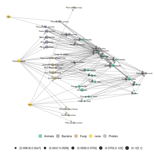
plot of chunk norway_attach_layout2
We see that even if the two layouts for the same \(\beta\) value are different, they share some structural characteristics. For example, fungal and bacterial groups are clustered together and are linked to their corresponding consumers (fungivore and bacterivore).
#attaching 'TL-tsne' layout to metaweb at class level
meta_norway = attach_layout(metanetwork = meta_norway,g = meta_norway$metaweb_trophic_class,beta = 0.006)
ggmetanet(g = meta_norway$metaweb_trophic_class,beta = 0.006,metanetwork = meta_norway)
plot of chunk norway_attach_layout3
‘group-TL-tnse’ layout
A variation of 'TL-tsne' layout consists in
'group-TL-tsne' layout. It mixes 'TL-tsne' and
a regular igraph layout to provide a representation where
species from the same group are clustered together. Such approach
provides more stable and interpretable. Morever, it is more efficient in
terms of computation time since it only requires 'TL-tsne'
layout computation at the aggregated level instead of computing it in
higher dimension at the group level. 'group-TL-tsne' layout
is stored as node attribute.
meta_norway = attach_layout(meta_norway,beta = 0.2,mode = "group-TL-tsne",res = "trophic_class")
vertex_attr_names(meta_norway$metaweb)
## [1] "name" "ab" "TL" "layout_beta0.006" "layout_beta0.006_1" "group_layout_x_beta0.2"
## [7] "group_layout_y_beta0.2"
ggmetanet(meta_norway,beta = 0.2,mode = "group-TL-tsne",legend = "trophic_class",ggnet.config = ggnet.custom)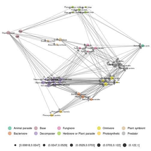
plot of chunk norway_metaweb_group_TL_tsne
Representing and comparing local networks
diff_plot allows comparing local networks. Here, it
provides a comparison between high and low disturbed sites by moth
outbreaks.
diff_plot(g1 = meta_norway$high,g2 = meta_norway$low,beta = 0.006,metanetwork = meta_norway)## mode is TL-tsne## plotting: high_trophic_group - low_trophic_group## mode is TL-tsne## beta = 0.006## Epoch: Iteration #100 error is: 1333.49922010638## Epoch: Iteration #200 error is: 319.518122109745## Epoch: Iteration #300 error is: 319.65237149482
plot of chunk norway_diffplot
It highlights a shift from Ectomycorrhizae and Ericoid mycorrhizae towards Arbuscular mycorrhizae due to increase of shrubs after the perturbation and also an increase in soil predator abundances. Here, a new ‘TL-tsne’ layout is computed.
Using metaweb layout
In order to gain reproducibility and not to compute
'TL-tsne' layout at each call, use argument
layout_metaweb = T to represent the difference network with
metaweb layout.
diff_plot(g1 = meta_norway$high,g2 = meta_norway$low,beta = 0.006,metanetwork = meta_norway,layout_metaweb = T)## mode is TL-tsne## plotting: high_trophic_group - low_trophic_group## mode is TL-tsne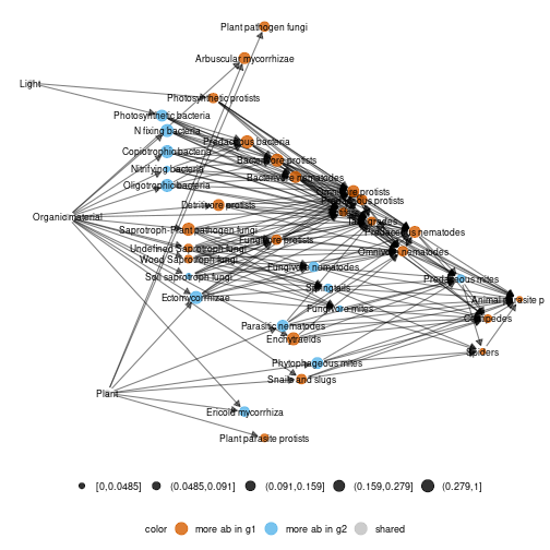
plot of chunk norway_diff_plot
Using 'group-TL-tsne' layout
Once computed on the metaweb, 'group-TL-tsne' layout can
be used in 'diff_plot'
ggnet.custom$arrow.size = 2
ggnet.custom$edge.alpha = 0.2

diff_plot(g1 = meta_norway$high,g2 = meta_norway$low,beta = 0.2, mode = "group-TL-tsne",
          metanetwork = meta_norway,layout_metaweb = T,ggnet.config = ggnet.custom)
## mode is group-TL-tsne## plotting: high_trophic_group - low_trophic_group## mode is group-TL-tsne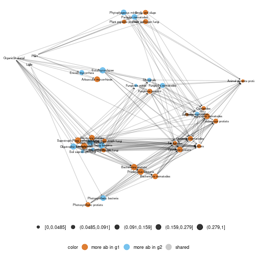
plot of chunk norway_diffplot_group_layout
Computing network indices and metrics
Besides network representation, ‘metanetwork’ package can compute usual network metrics (weighted connectance, mean and max trophic level, mean shortest path length). Network diversity and dissimilarity indices based on Hill numbers are also implemented in order to quantitatively compare local networks at the different resolutions.
metrics_norway = compute_metrics(meta_norway)## Error in t(igraph::V(g)$ab) %*% adj: arguments inadéquats
#metrics at the different resolutions
metrics_norway$trophic_group
## Error in eval(expr, envir, enclos): objet 'metrics_norway' introuvable
metrics_norway$trophic_class## Error in eval(expr, envir, enclos): objet 'metrics_norway' introuvable
metrics_norway$taxa## Error in eval(expr, envir, enclos): objet 'metrics_norway' introuvableWe now compute network diversity indices based on Hill numbers
(cf. Ohlmann et al. 2019). The indices are based on node and link
abundances are can be partitioned in \(\alpha\)-diversity, \(\beta\)-diversity and \(\gamma\)-diversity. A viewpoint parameter
\(q\) allows giving more weight (see
compute_div documentation)
div_norway = compute_div(meta_norway)

div_norway$nodes
## trophic_group trophic_class taxa
## Gamma_P 17.166819 4.637323 3.865180
## mean_Alpha_P 16.645513 4.600212 3.847461
## Beta_P 1.031318 1.008067 1.004605
## Alpha_high_P 17.833549 4.650241 3.924770
## Alpha_low_P 15.536622 4.550721 3.771674
div_norway$links## trophic_group trophic_class taxa
## Gamma_L 52.899140 8.044432 9.227551
## mean_Alpha_L 48.298149 7.918602 9.093270
## Beta_L 1.095262 1.015890 1.014767
## Alpha_high_L 63.542723 8.410311 9.868439
## Alpha_low_L 36.710910 7.455640 8.378992As reported in Calderon-Sanou et al. 2021, we see higher node and
link diversities in sites with a high perturbation level. This is due to
the fact that dominant groups tend to to disappear, giving way to an
increase in predator groups and leading so to more evenly distributed
abundances. Pairwise dissimilarity indices (both on nodes and links) are
also implemented in metanetwork (see compute_dis
documentation).
dis_norway = compute_dis(meta_norway)

#nodes and links dissimilarity at Species resolution
dis_norway$trophic_group$nodes
## high low
## high 0.00000000 0.04448943
## low 0.04448943 0.00000000
dis_norway$trophic_group$links## high low
## high 0.0000000 0.1312764
## low 0.1312764 0.0000000
#nodes and links dissimilarity at Phylum resolution
dis_norway$trophic_class$nodes
## high low
## high 0.00000000 0.01159194
## low 0.01159194 0.00000000
dis_norway$trophic_class$links## high low
## high 0.00000000 0.02274482
## low 0.02274482 0.00000000
#compute dissimilarity at taxa resolution only
compute_dis(meta_norway,res = "taxa")
## $taxa
## $taxa$nodes
## high low
## high 0.000000000 0.006628866
## low 0.006628866 0.000000000
##
## $taxa$links
## high low
## high 0.00000000 0.02114852
## low 0.02114852 0.00000000We see that networks are more dissimilar at trophic_group compared to
trophic_class resolution both on nodes and links. Moreover, at both
resolutions, network are more dissimilar regarding link abundances
compared to node abundances. To gain in efficiency,
compute_dis is uses parallel computation (see
ncores argument in compute_dis
documentation)
References
Calderón-Sanou, I., Münkemüller, T., Zinger, L., Schimann, H., Yoccoz, N. G., Gielly, L., … & Thuiller, W. (2021). Cascading effects of moth outbreaks on subarctic soil food webs. Scientific Reports, 11(1), 15054.
Ohlmann, M., Miele, V., Dray, S., Chalmandrier, L., O’connor, L., & Thuiller, W. (2019). Diversity indices for ecological networks: a unifying framework using Hill numbers. Ecology letters, 22(4), 737-747.