Angola data set
An example using real data is accessible in metanetwork. It consists in the Angoala coastal trophic network from Angelini, R. & Vaz-Velho, F. (2011)., abundance data at different time steps (1986 and 2003) and a trophic table, indicating the groups to which species belong.
Loading the dataset
## [1] "metanetwork"
print(meta_angola)## metaweb has 28 nodes and 127 edges
## 2 local networks
## available resolutions are: Species Phylum
plot_trophic_table function
Contrary to the pyramid example, angola dataset do have a trophic
table, describing nodes memberships in higher relevant groups. In angola
dataset, two different taxonomic resolutions are available. Networks can
be handled and represented at Species or Phylum level.
The plot_trophic_table function allows representing the
tree describing species memberships.
ggnet.custom = ggnet.default
ggnet.custom$label.size = 2
plot_trophicTable(meta_angola,ggnet.config = ggnet.custom)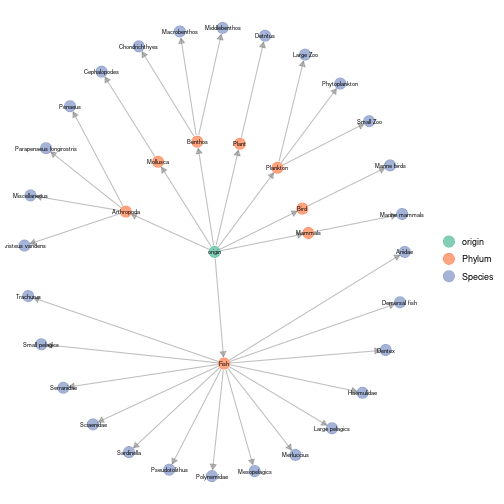
plot of chunk angola_plot_trophicTable
append_agg_nets method
The method append_agg_nets allows computing and
appending aggregated networks (at the different available resolutions)
to the current metanetwork.
meta_angola = append_agg_nets(meta_angola)
print(meta_angola)
## metaweb has 28 nodes and 127 edges
## 2 local networks
## available resolutions are: Species PhylumRepresenting aggregated networks, adding a legend to networks
Once computed, ggmetanet function allows representing
aggregated networks and legending local networks using trophic table. Do
not forget to first compute trophic levels.
meta_angola = compute_TL(meta_angola)
ggmetanet(g = meta_angola$metaweb_Phylum,beta = 1,metanetwork = meta_angola)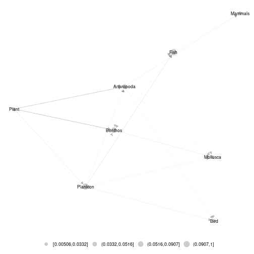
plot of chunk angola_metaweb_phylum
Node sizes are proportional to relative abundances. Trophic table allows adding a legend to network at the finest resolution.
ggmetanet(g = meta_angola$metaweb,beta = 0.04,legend = 'Phylum',metanetwork = meta_angola)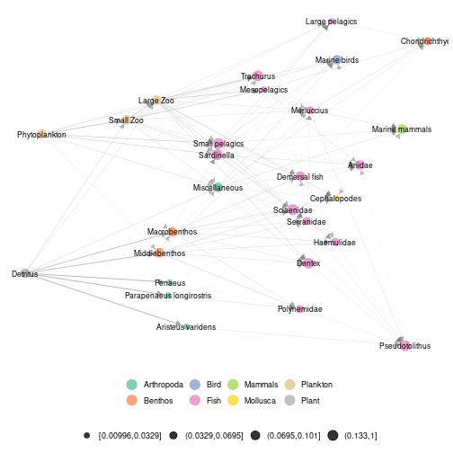
plot of chunk angola_metaweb
The metaweb has two basal nodes, ‘Phytoplankton’ and ‘Detritus’, leading to a primary producer and detritus channel that mix up higher in the network. The ‘TL-tsne’ layout highlights these two distinct channels for both networks: the green channel, linked to primary producers, (phytoplankton) and the brown channel, linked to detritus.
diff_plot
To represent difference between local networks, use
diff_plot() function.
diff_plot(g1 = meta_angola$X1986,g2 = meta_angola$X2003,beta = 0.04,metanetwork = meta_angola)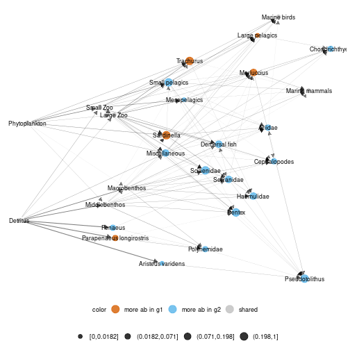
plot of chunk angola_diff_plot
vismetaNetwork function
metanetwork allows representing trophic networks in interactive way
using visNetwork function and both layout algorithms. We
highly recommend this function to explore large and dense networks.
Since outputs of this functions cannot be rendered on this README, they
are saved in ./vismetaNetwork in html format.
x_y_range argument allows controlling the x-axis and y-axis
scale.
vismetaNetwork(metanetwork = meta_angola,beta = 0.04,legend = 'Phylum',x_y_range = c(30,60))Interactive visualisation of angola dataset and other trophic
networks using vismetaNetwork are available at https://shiny.osug.fr/app/ecological-networks.
Additional features
attach_layout function
Since TL-tsne layout is stochastic and requires (a bit
of) computation times, saving and using the the same layout (for a given
\(\beta\) value) is recommended.
Moreover, it makes easier visual network analysis and comparison since
it is fixed. attach_layout function allows saving computed
layouts by attaching them as a node attribute.
#attaching a layout to the metaweb
meta_angola = attach_layout(metanetwork = meta_angola,beta = 0.05)
#layout is saved as node attribute (only one component since the other one is trophic level)
igraph::vertex_attr_names(meta_angola$metaweb)
## [1] "name" "ab" "TL" "layout_beta0.05"
#this is the computed layout
V(meta_angola$metaweb)$layout_beta0.05
## [1] -9.651342 -5.767532 5.194469 -3.823952 -18.572339 15.773919 21.064580 7.543386 25.917790 23.226553 11.649604 29.426068 -16.106680
## [14] -21.246919 -27.047448 -1.600164 -23.833696 2.788126 0.646412 18.443714 -14.331872 -31.772174 9.648135 13.705864 -7.831115 -12.831562
## [27] -10.993820 20.381996
#ggmetanet uses the computed layout
ggmetanet(meta_angola,beta = 0.05,legend = "Phylum")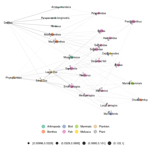
plot of chunk angola_attach_layout1
Several layout can be computed and stored for the same \(\beta\) value. Argument
nrep_ly allows selecting the desired computed layout for
the focal \(\beta\) value.
#attaching a new layout for the same beta value
meta_angola = attach_layout(metanetwork = meta_angola,beta = 0.05)
#the two layouts are stored as node attribute
igraph::vertex_attr_names(meta_angola$metaweb)
## [1] "name" "ab" "TL" "layout_beta0.05" "layout_beta0.05_1"
#this is the new layout
V(meta_angola$metaweb)$layout_beta0.05_1
## [1] 23.2884614 4.1340300 -4.8161359 15.5999164 10.4074526 -15.3107874 -20.5228096 -7.1625291 -25.3092535 -22.6558866 -11.2409679 -28.7714286
## [13] 13.2750092 18.0097423 26.7344642 1.9609046 20.4578198 -2.4228296 -0.2968211 -17.9566698 7.4907073 31.4329101 -9.2597165 -13.2684559
## [25] 6.1029551 8.6541160 11.3126872 -19.8668844
#ggmetanet with the new 'TL-tsne' layout
ggmetanet(meta_angola,beta = 0.05,legend = "Phylum",nrep_ly = 2)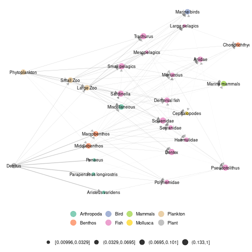
plot of chunk angola_attach_layout2
Notice that even if the two layouts are quite different in term of global structure, they share some features in terms of local structure. For example, phytoplankton and zooplankton are close by as Detritus and benthic organisms. So, in this example, despite the stochasticity of the layout, the highlight of brown and green channels is stable.
Using metaweb layout
Using metaweb layout can ease the representation and comparison of multiple local networks.
#using metaweb layout to represent a local network
ggmetanet(g = meta_angola$X1986,metanetwork = meta_angola,
          legend = "Phylum",layout_metaweb = T,beta = 0.05)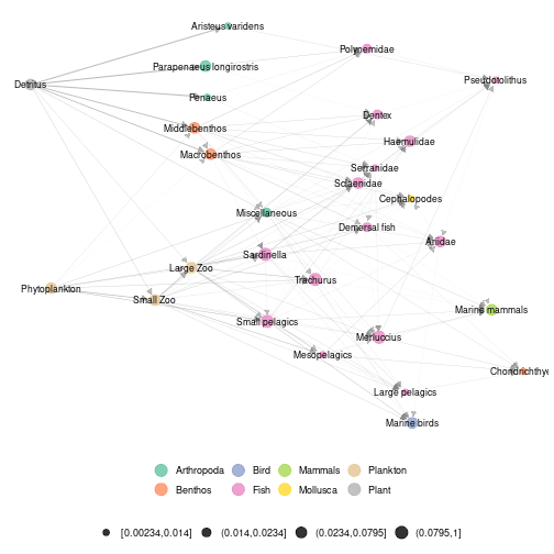
plot of chunk angola_layout_metaweb
#using metaweb layout for diffplot
diff_plot(g1 = meta_angola$X1986,g2 = meta_angola$X2003,
          metanetwork = meta_angola,beta = 0.05,
          layout_metaweb = T)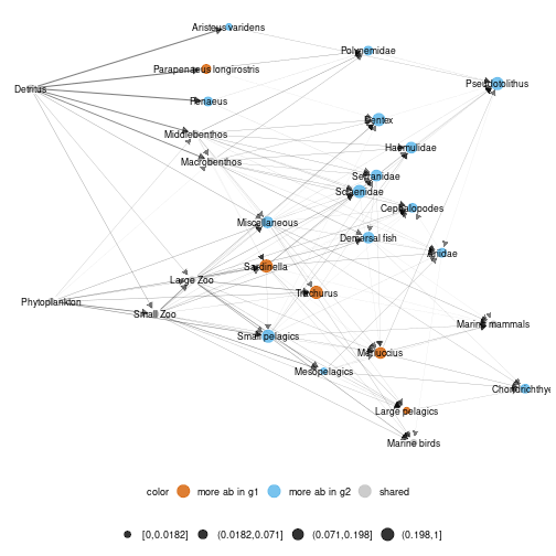
plot of chunk angola_layout_metaweb
Computing network indices and metrics
Besides network representation, ‘metanetwork’ package can compute usual network metrics (weighted connectance, mean and max trophic level, mean shortest path length). Network diversity and dissimilarity indices based on Hill numbers are also implemented in order to quantitatively compare local networks at the different resolutions.
metrics_angola = compute_metrics(meta_angola)
metrics_angola$Species
## connectance mean_TL max_TL mean_shortest_path_length
## metaweb 0.02921234 1.561919 2.739126 0.2201667
## X1986 0.02859672 1.561919 2.739126 0.2201667
## X2003 0.02918298 1.561919 2.739126 0.2201667
metrics_angola$Phylum## connectance mean_TL max_TL mean_shortest_path_length
## metaweb 0.02925731 1.315389 2.229886 0.05117634
## X1986 0.02859672 1.319967 2.278338 0.04603361
## X2003 0.02918298 1.317792 2.206484 0.05471144We now compute network diversity indices based on Hill numbers
(cf. Ohlmann et al. 2019). The indices are based on node and link
abundances are can be partitioned in \(\alpha\)-diversity, \(\beta\)-diversity and \(\gamma\)-diversity. A viewpoint parameter
\(q\) allows giving more weight (see
compute_div documentation)
div_angola = compute_div(meta_angola, q = 1)
div_angola$nodes
## Species Phylum
## Gamma_P 13.666059 2.680737
## mean_Alpha_P 12.478328 2.669698
## Beta_P 1.095183 1.004135
## Alpha_X1986_P 9.027714 2.494158
## Alpha_X2003_P 17.247852 2.857593
div_angola$links## Species Phylum
## Gamma_L 54.570083 3.812301
## mean_Alpha_L 47.556571 3.791652
## Beta_L 1.147477 1.005446
## Alpha_X1986_L 35.532836 3.410505
## Alpha_X2003_L 63.648943 4.215394We see a higher \(\alpha\)-diversity
in 2003 compared to 1986 both on nodes and links and both at Species and
Phylum resolution. Moreover, pairwise dissimilarity indices (both on
nodes and links) are also implemented in metanetwork (see
compute_dis documentation).
dis_angola = compute_dis(meta_angola)

#nodes and links dissimilarity at Species resolution
dis_angola$Species$nodes
## X1986 X2003
## X1986 0.0000000 0.1311726
## X2003 0.1311726 0.0000000
dis_angola$Species$links## X1986 X2003
## X1986 0.0000000 0.1984655
## X2003 0.1984655 0.0000000
#nodes and links dissimilarity at Phylum resolution
dis_angola$Phylum$nodes
## X1986 X2003
## X1986 0.000000000 0.005952805
## X2003 0.005952805 0.000000000
dis_angola$Phylum$links## X1986 X2003
## X1986 0.000000000 0.007835491
## X2003 0.007835491 0.000000000
#compute dissimilarity at Phylum resolution only
compute_dis(meta_angola,res = "Phylum")## $Phylum
## $Phylum$nodes
##             X1986       X2003
## X1986 0.000000000 0.005952805
## X2003 0.005952805 0.000000000
##
## $Phylum$links
##             X1986       X2003
## X1986 0.000000000 0.007835491
## X2003 0.007835491 0.000000000We see that networks are more dissimilar at Species compared to
Phylum resolution both on nodes and links. Moreover, at both
resolutions, network are more dissimilar regarding link abundances
compared to node abundances. To gain in efficiency,
compute_dis uses parallel computation (see
ncores argument in compute_dis
documentation)
References
Angelini, R., & Vaz-Velho, F. (2011). Ecosystem structure and trophic analysis of Angolan fishery landings. Scientia Marina(Barcelona), 75(2), 309-319.
Ohlmann, M., Miele, V., Dray, S., Chalmandrier, L., O’connor, L., & Thuiller, W. (2019). Diversity indices for ecological networks: a unifying framework using Hill numbers. Ecology letters, 22(4), 737-747.